One Poem Suffices: Basic LLM Inference and Generation

0. Goal

This post aims to answer two questions, with all inference operations explained by cross-referencing the meta-llama codebase.

• Question 1: Given N input tokens (a prompt), how does an LLM get the next token? And how does it perform auto-regressive sampling?
• Question 2: How does an LLM handle variable-length batch inference?

1. Pre-Knowledge

1.1. Temperature

Before running generation, the model sometimes requires a temperature value. What is it, and what does it do?

Usually, the model outputs raw values (logits) rather than a probability distribution, so we need to convert them into a distribution, typically using the Softmax function:

$$\dfrac{\exp(z_i)}{\sum \exp(z_j)}$$

Although Softmax gives us a distribution, it also has drawbacks. It tends to amplify or shrink differences among the internal elements, degenerating toward max or mean. For example (borrowed from another explanation):

• Applying Softmax to [11, 12, 13] yields [0.0900, 0.2447, 0.6652], which makes the final sampled results lack diversity.

• Applying Softmax to [0.01, 0.02, 0.03] yields [0.3300, 0.3333, 0.3367], which turns the final sampling step into nearly uniform random sampling and generates unreasonable sequences.

Temperature T is used to solve this problem by adjusting Softmax so that the resulting distribution better matches our expectations.

$$\dfrac{\exp(z_i / T)}{\sum \exp(z_j / T)}$$

As shown below, this animation helps us quickly understand how $T$ affects the Softmax distribution.

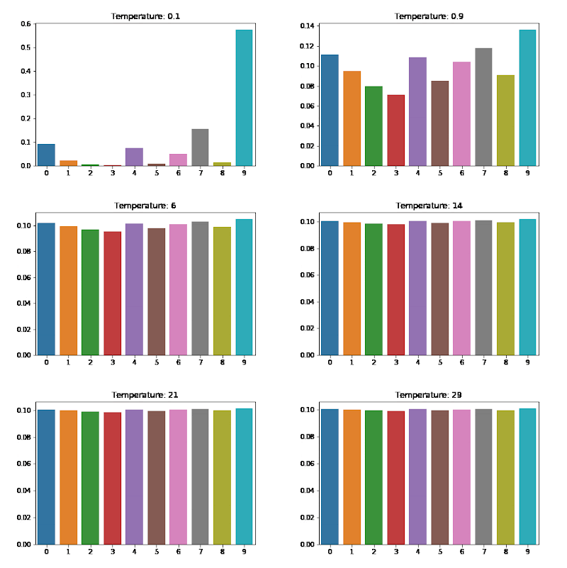
• As $T$ increases, the distribution approaches a uniform distribution, and the sampled results become more random.
• As $T$ decreases, the distribution approaches a one-point distribution, and the sampled results become more deterministic.

So why is it called temperature? As we know, the higher the temperature, the more vigorous the Brownian motion; similarly, the higher the temperature, the more random the sampled results.

1.2. Top-p/Nucleus Sampling

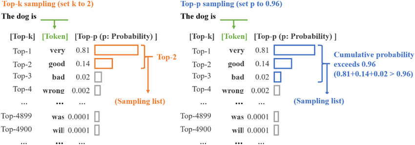
The core idea of top-p sampling is to select the smallest set of tokens whose cumulative probability exceeds a threshold p, and then randomly sample the next token from this set. This set is called the nucleus, which is also where the name nucleus sampling comes from.

The diagram below illustrates the whole workflow (on the right): after selecting the nucleus set, we re-normalize the probabilities and then sample from them. If top-p sampling still feels unclear, you can refer to the sample_top_p implementation in llama2 (linked here in a version with Chinese comments).

2. Learn by llama code

2.1. generate function signature

There are already many explanations of the entire llama repository online. To differentiate this post and make it smoother to read, I will focus only on the generate function relevant to our topic. I will also omit parts of the code that do not affect the narrative flow, rather than explaining the code line by line in the article (I plan to create a dedicated repo to help with learning meta-llama).

First, let's look at the function signature:

• torch.inference_mode(): You can think of this as an optimization similar to torch.no_grad(), used to speed up inference.
• prompt_tokens: A 2D list storing the token IDs of the tokenized prompts. The first dimension represents the batch size.
• max_gen_len: The maximum length of the generated text sequence.
• temperature: See the introduction above. Used to control sampling randomness.
• top_p: Likewise, see the introduction above. Used to set the threshold for top-p sampling.
• We can skip the remaining parameters, as they are not important for this post.

@torch.inference_mode()
def generate(
    self,
    prompt_tokens: List[List[int]],
    max_gen_len: int,
    temperature: float = 0.6,
    top_p: float = 0.9,
    logprobs: bool = False,
    echo: bool = False,
) -> Tuple[List[List[int]], Optional[List[List[float]]]]:

2.2. Goal1: How to auto-regressive sampling?

prompt_tokens is 2D because it is designed for batch inference. Let's break the problem down and start with the simplest case: suppose prompt_tokens is a 1D sequence. What does auto-regressive sampling look like in that case?

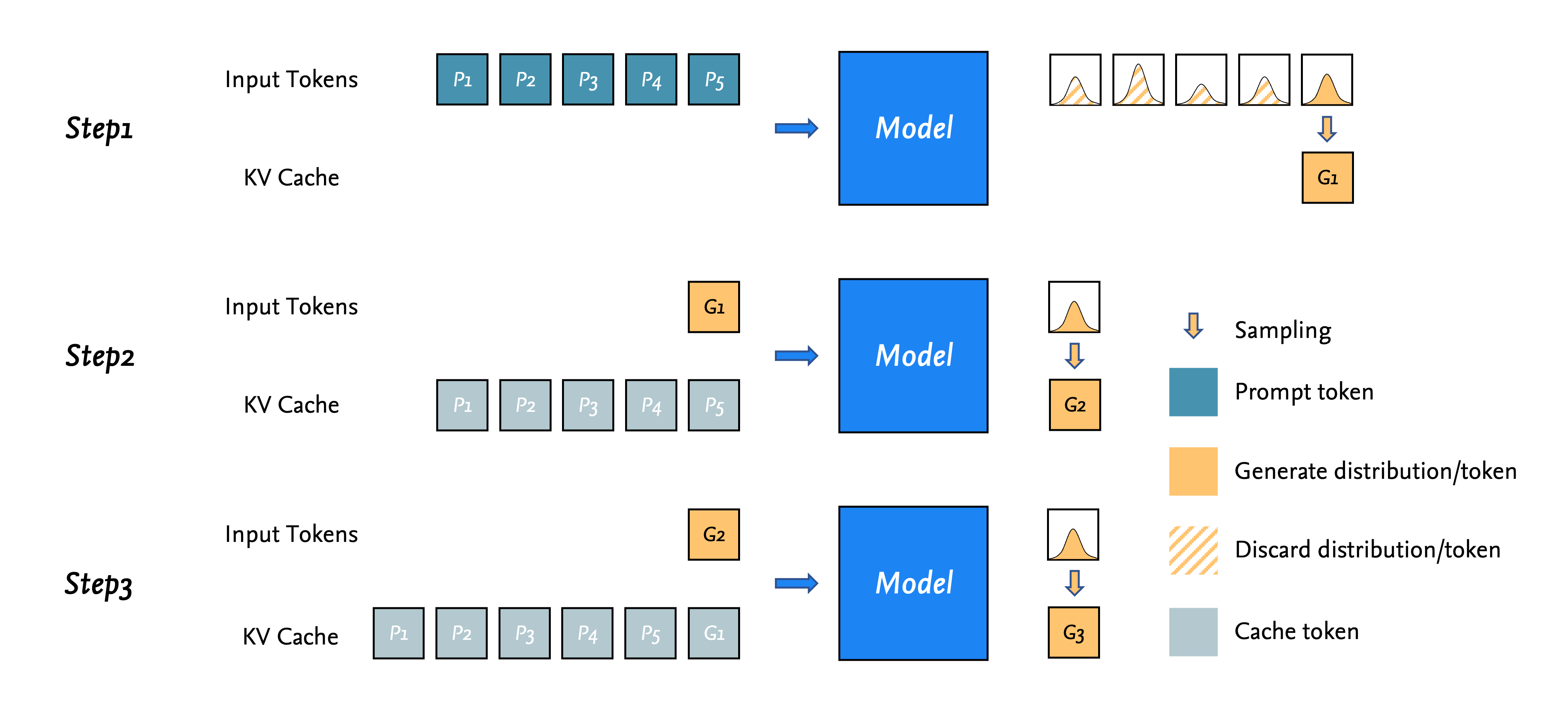
A picture is worth a thousand words, and people learn more efficiently from visuals, so let's analyze this with the diagram below. Suppose we have $N$ tokens:

1. In the first step, the $N$ prompt tokens are fed into the model at the same time, producing $N$ distributions (for predicting the next token). Only the last one is the distribution we need; the other computed distributions are ignored. (Right side of Step 1 in the figure: only the last distribution goes through further sampling.)
2. At the same time, part of the computation results for the prompt tokens fed into the model is cached in the KV cache (gray blocks on the left of Step 2 in the figure), so subsequent auto-regressive sampling steps only need to take the token predicted in the previous sampling step to complete the computation.
3. Repeat this process until the model generates a token representing the end of generation or the generated sequence exceeds the maximum sequence length set for the model.

2.3. Goal2: How to batch inference?

In Goal 1, we understood auto-regressive sampling without batching. Next, let's try to answer the second and final question: how does an LLM handle variable-length batch inference? Keep in mind that we are covering basic inference here, so this is the simplest case; modern inference libraries certainly apply all kinds of optimizations (which we will try to unpack step by step in future posts).

Suppose the input prompt_tokens has a batch size of B, and the sequences do not necessarily have the same length.

We focus on two lengths: min_prompt_length and total_length. The first is easy to understand: it is the sequence length of the shortest prompt in the input batch. The second is slightly more involved: it represents the maximum possible length in the batch.

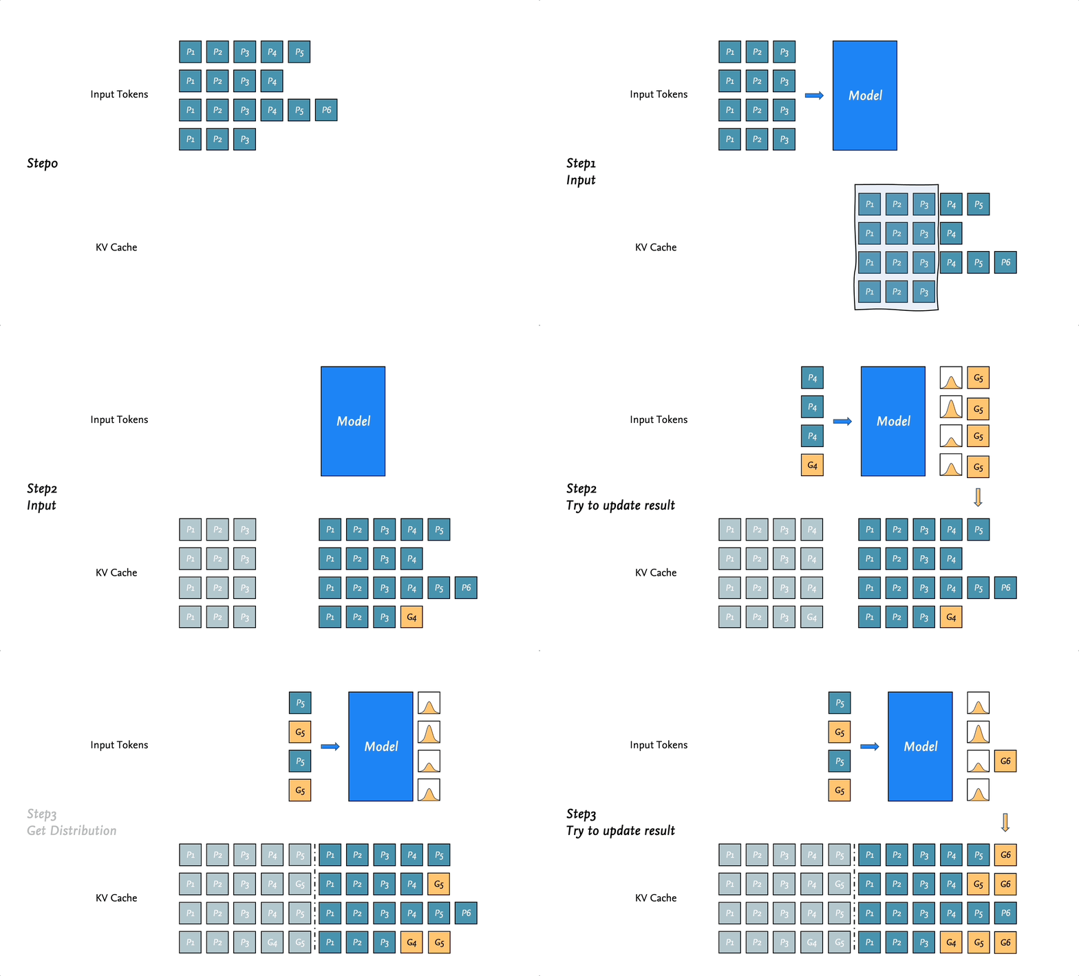
Now comes the first key point: which position should we start generating from? Ideally, every sequence in the batch would start generating its next token right after its own prompt, with nothing wasted (at first I even wondered if that was how it worked, haha). However, the model has to process tensors of the same length, and we cannot guarantee that all sequences in the batch have the same length. Therefore, batch inference initially starts generating from min_prompt_length (see Step 1 in the animation).

After that, the workflow is relatively straightforward. Referring back to Goal 1, except for the first inference step, each subsequent inference step only needs to take a token sequence of shape [B, 1].

The only difference is that in Goal 1, the token finally sampled by the model is always one we need. In batch inference, however (see Steps 1/2/3 in the animation), because we have to start generating from min_prompt_length, if the current position already has a user-provided token, the token sampled by the model is discarded.

To summarize the main differences compared with non-batch inference:

• We need to account for min_prompt_length in the batch, so inference efficiency is naturally constrained by it (consider one prompt of length $1$ token and three prompts of length $100$ tokens). An uneven sequence length distribution in the batch can severely limit inference performance. In batch inference, generated tokens may be invalid and wasted.

Once we understand how an LLM performs batch inference, we can also see that this paradigm involves substantial redundant computation and wasted performance, leaving plenty of room for optimization. This is the inevitable reason Continuous batching was later introduced.

References

• Blog: A Walkthrough of LLM Inference
• Github Repo: meta-llama/llama
• Github Repo: keli-wen/meta-llama2-explain
• TORCH.MULTINOMIAL
• Blog: A 2023 Beginner's Guide to Deep Learning (19) - LLaMA 2 Source Code Analysis

Next Read

• Continuous batching.
• KV Cache in LLM.